
Reddit Between the Lines: Unveiling Subreddit Topics
Reddit Between the Lines
Executive Summary
The objective of this study is to find clusters or ‘subreddits’ among Reddit articles and provide relevant insights or trends that will help identify customer behavior. From a sample data provided, data mining techniques were used to prepare the data for analysis. Unsupervised clustering techniques such as K-means clustering were used to determine the optimum number of clusters of the dataset. NLTK Vader Analyzer was also used to identify and categorize Reddit titles into three sentiments: positive, negative, or neutral. K-means clustering generated an optimal number of cluster equal to 7 using Internal Validation Criteria: Sum of squares distances to centroids, Calinski-Harabasz index, Intracluster to intercluster distance ratio, Silhouette coefficient. The general topics generated were Online Recommendations, The Democrats, Today I Learned, Customer Support, Gaming, New Year and Donald Trump. From the sentiment analysis, it was found out that 64.5% of the titles have neutral tone, while 23.54% of the titles have negative tone and 11.94% of the titles have positive tone. Findings of the study can be used in enhancing the subreddit tagging to avoid subreddits having similar discussion points however, further processing of dataset such as lemmatization and stemming is recommended to generate more significant results.
Methodology
To meet the said objectives of the study, dataset from Reddit, comprised of titles and authors, will be used in the analysis. Python programming language will be used in extracting, wrangling and analysis of the data. From the available dataset, exploratory data analysis will then be conducted to determine which data wrangling method to use in cleaning the data. Cleaned and processed data will be used in K-means clustering and sentiment analysis using NLTK. From the two methods specified, clusters and insights will be generated. Details of each method will be explained in a separate section below.
Python Libraries
The following libraries and modules will be used:
import pandas as pd
import numpy as np
import seaborn as sns
import random
import matplotlib.pyplot as plt
import re
from sklearn.preprocessing import StandardScaler
from sklearn.feature_extraction.text import TfidfVectorizer
from scipy.spatial.distance import euclidean
from sklearn.metrics import calinski_harabaz_score, silhouette_score
from sklearn.manifold import TSNE
from sklearn.decomposition import TruncatedSVD
from scipy.spatial.distance import euclidean, cityblock
from wordcloud import WordCloud, ImageColorGenerator
from sklearn.cluster import KMeans
from os import path, getcwd
from PIL import Image
import collections
from nltk.tokenize import word_tokenize, RegexpTokenizer
from nltk.corpus import stopwords
from IPython.display import HTML
Data Description
Data sample consists of post titles (with authors when available) from Reddit. Reddit is a social news aggregation, web content rating, and discussion website. It is considered as “the front page of the internet, where everything surfaces. “The site splits up posts into different subject sections called “subreddits”. Users (authors) start a conversation by posting a topic under a subreddit, which is also referred as the title. The Reddit community reacts to the post by upvoting, downvoting, commenting and sharing.
Usually, the title itself attracts the attention of online users however, Reddit may appear to be messy sometimes due to duplication or similarity of subreddits making “everything all over the place”. In posting a new topic, a user specifies the subreddit without any strict rules. He/she can just click any subreddit and continue with the post. This project aims to cluster different subreddit titles and generate some insights that might help developers on how to properly group posts on the website. By clustering the titles, a better subreddit might be generate since words having similar features will be grouped together.
Data Processing
The provided dataset is an example of unstructured data extracted from the web. In order to have a sound analysis, data needs to be transformed into a uniformed structure.
Pre-Processing: This process would involve doing exploratory data analysis, cleaning and transforming the dataset to a uniformed structure by removing punctuations and non-ASCII characters, lowering alphanumeric characters, removing stopwords. The output of this process would allow easier processing of data. For example, if stopwords such as ‘the’, ‘a’, ‘of’ were included in the dataset, a good analysis will not be made.
Vectorizing: Since the dataset type is text, clustering cannot process text directly. Text should be converted to numbers using Term Frequency — Inverse Data Frequency (TF-IDF) technique. TF-IDF standardizes the textual data by assigning weights on words depending on how frequent a word is used and produces the “Bag of Words” Model.
Clustering: Two types of clustering will be conducted to analyze the processed dataset: K-means clustering and NLTK’s vader analyzer. K-means algorithms is fast to execute, computing the distances between points and group centers which is why it was chosen as the method of analysis. NLTK’s vader analyzer classifies the titles into three sentiments: positive, negative, or neutral.
Validation: To validate the number of clusters in the K-means clustering, internal validation criteria will be used to determine the optimal number of clusters.
Opening the Dataset
Data sample was saved in a .txt file. In order to access the contents of the file, Pandas read_csv library will be used.
df = pd.read_csv('reddit-dmw-sample.txt', sep="\t")
df.head()
| Unnamed: 0 | author | title | |
|---|---|---|---|
| 0 | 0 | PrimotechInc | 7 Interesting Hidden Features of apple ios9 |
| 1 | 1 | xvagabondx | Need an advice on gaming laptop |
| 2 | 2 | nkindustries | Semi automatic ROPP Capping machine / ROPP Cap... |
| 3 | 3 | Philo1927 | Microsoft Plumbs Ocean’s Depths to Test Underw... |
| 4 | 4 | tuyetnt171 | OPPO F1 chính hãng - Fptshop.com.vn |
The file contains three columns- index, author and title of the article. The first column will be dropped since it is just the same with the index of the DataFrame.
df = df.drop(axis= 1, columns= 'Unnamed: 0')
df.head()
| author | title | |
|---|---|---|
| 0 | PrimotechInc | 7 Interesting Hidden Features of apple ios9 |
| 1 | xvagabondx | Need an advice on gaming laptop |
| 2 | nkindustries | Semi automatic ROPP Capping machine / ROPP Cap... |
| 3 | Philo1927 | Microsoft Plumbs Ocean’s Depths to Test Underw... |
| 4 | tuyetnt171 | OPPO F1 chính hãng - Fptshop.com.vn |
df.describe()
| author | title | |
|---|---|---|
| count | 6000 | 6000 |
| unique | 3869 | 5856 |
| top | [deleted] | Kindle Fire Phone Number 1-844-801-7563 |
| freq | 1187 | 9 |
Looking intially at the dataset, we have 6000 samples. However, it can be observed that we have a lot of duplicate titles and deleted authors. Note that this data is still unstructured and not uniform since punctuations are non-uniform cases are present.
Cleaning
Data wrangling techniques will be used to clean and make the data uniform. First is to remove non-ASCII characters on all title entries since one of the limitations of using vectorizer is it can only remove English stopwords.
# filter
words = []
for i in df['title'].tolist():
    if i.encode("ascii", errors="ignore").decode() != "":
        words.append(i.encode("ascii", errors="ignore").decode().strip())
To store the processed text, new DataFrame is created.
df_new = pd.DataFrame(words,columns=['title_lower'])
df_new.head()
| title_lower | |
|---|---|
| 0 | 7 Interesting Hidden Features of apple ios9 |
| 1 | Need an advice on gaming laptop |
| 2 | Semi automatic ROPP Capping machine / ROPP Cap... |
| 3 | Microsoft Plumbs Oceans Depths to Test Underwa... |
| 4 | OPPO F1 chnh hng - Fptshop.com.vn |
The punctuations will now be removed.
df_new['title_lower'] = df_new['title_lower'].str.replace('[^\w\s]','')
df_new.head()
| title_lower | |
|---|---|
| 0 | 7 Interesting Hidden Features of apple ios9 |
| 1 | Need an advice on gaming laptop |
| 2 | Semi automatic ROPP Capping machine ROPP Cap ... |
| 3 | Microsoft Plumbs Oceans Depths to Test Underwa... |
| 4 | OPPO F1 chnh hng Fptshopcomvn |
To make the words uniform, all texts in the title will be transformed to lower case.
df_new["title_lower"] = df_new['title_lower'].str.lower()
df_new.head()
| title_lower | |
|---|---|
| 0 | 7 interesting hidden features of apple ios9 |
| 1 | need an advice on gaming laptop |
| 2 | semi automatic ropp capping machine ropp cap ... |
| 3 | microsoft plumbs oceans depths to test underwa... |
| 4 | oppo f1 chnh hng fptshopcomvn |
Exploratory Data Analysis
Now that the dataset has uniform structure, exploratory data analysis will be performed. After the pre-processing, the number of unique title entries were reduced to 5800 from 5856. There was also 1 entry which was discarded due to non-ASCII characters. There were also 25 titles which have non-alphanumeric characters that were replaced with blanks.
df_new.describe()
| title_lower | |
|---|---|
| count | 5999 |
| unique | 5800 |
| top | |
| freq | 25 |
One of the easiest way to analyze the data is obtaining most commonly discussed topics by different authors.
title_list = df_new['title_lower'].tolist()
counter = collections.Counter(title_list)
for x, y in counter.most_common(10):
    print(x, ": ", y)
 :  25
kindle fire phone number 18448017563 :  9
steven mandell :  8
inside the clintons plan to defeat donald trump :  7
happy new year reddit  i quit retirement spent 250k in savings and 51 months 15000 hours to develop the new internet owned by the people powered by humanity  the first company in history equally owned by everybody alive we are uniting the whole world into one :  5
phases of web development process :  5
dual usb travel chargers by slanzer technology  convenience optimized :  4
microsoft plumbs oceans depths to test underwater data center :  3
donald trumps strongest supporters a certain kind of democrat :  3
trump to chris christie get in the plane you go home :  3
The output above shows the top 10 titles with duplicates. Note that the highest number of duplicates are the titles with non-ASCII characters amounting to 25 entries.
Finding a simmilarities on the topics above can be difficult since by looking at the title alone, insufficient insights can be generated. Another way to quickly analyze the dataset is to breakdown the title into words and remove stop words. Stop words are considered irrelevant for searching purposes and natural text processing because they occur frequently in a sentence.
# define list of stopwords
def process_text(title):
    """
    Returns a list of strings without stop words from an input list of
    string.

    """
    tokens = []
    tokenizer = RegexpTokenizer(r'\w+')
    stop_words = stopwords.words('english')
    for line in title:
        toks = tokenizer.tokenize(line)
        toks = [t.lower() for t in toks if t.lower() not in stop_words]
        tokens.extend(toks)
    return tokens
Generating the most used words in the dataset:
# get the most common used words in the dataframe, removing stop words:
data_set = process_text(df_new['title_lower'].tolist())
string = " ".join(data_set)
Counter = collections.Counter(string.split())
most_occur = Counter.most_common(10)


# generate horiontal barplot:
fig, ax = plt.subplots(1, 2, figsize=(20, 6));
fig.suptitle('Most Common Used Words', fontsize=19);
ax[0].barh([x[0] for x in most_occur][::-1], [y[1] for y in most_occur][::-1],
           height=0.6, align='center', color=['grey', 'grey', 'grey', 'grey',
                                              'grey', 'grey', 'grey', 'grey',
                                              'grey', 'darkcyan']);
plt.sca(ax[0]);
plt.xticks(range(0, [y[1] for y in most_occur][0], 200));
ax[0].set_xlabel('word count');
ax[0].set_ylabel('word');

# generate word cloud:
d = getcwd()
mask = np.array(Image.open(path.join(d, "reddit_logo.png")))
reddit = WordCloud(max_font_size=50, max_words=600, mask=mask,
                   background_color="white", random_state=1500).\
    generate(' '.join(data_set))
image_colors = ImageColorGenerator(mask);
ax[1].imshow(reddit, interpolation='bilinear');
ax[1].axis("off");
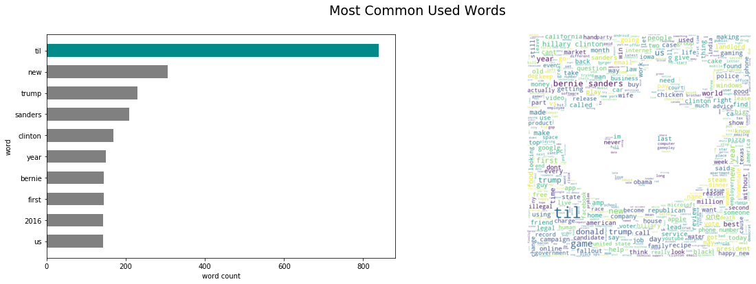
The barplot above shows the top 10 most frequently used words in the data set. The word til, abbreviation of ‘Today I Learned’, is the most frequently used word, appearing 839 times from the pool of 5999 titles.
The word cloud generated above shows a visual representation of the list of words found in the database, in which the size of each word indicates how frequent it was used in a document.
Vectorizing
Python sklearn library has a method TfidfVectorizer method that generates the term frequency matrix or bag of words (BoW). Words that occur frequently within a document but not frequently within the corpus receive a higher weighting as these words are assumed to contain more meaning in relation to the document. TfidfVectorizer can select words which follows a token pattern and remove stop words as shown below.
tfidf_vectorizer = TfidfVectorizer(token_pattern=r'[a-z-]+',
                                   stop_words='english')
bow_title = tfidf_vectorizer.fit_transform(df_new['title_lower'].tolist())
nonzeros = bow_title.sum(axis=1).nonzero()[0]
bow_title.todense()
matrix([[0., 0., 0., ..., 0., 0., 0.],
        [0., 0., 0., ..., 0., 0., 0.],
        [0., 0., 0., ..., 0., 0., 0.],
        ...,
        [0., 0., 0., ..., 0., 0., 0.],
        [0., 0., 0., ..., 0., 0., 0.],
        [0., 0., 0., ..., 0., 0., 0.]])
bow_title is the frequency matriz or BoW to be used in clustering.
X_title_new = TSNE(random_state=1337).fit_transform(
    TruncatedSVD(n_components=2000).fit_transform(bow_title))
plt.scatter(X_title_new[:,0], X_title_new[:,1], alpha=0.8);
plt.xlabel('dim 1');
plt.ylabel('dim 2');
plt.title('TSNE Plot');
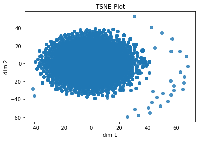
The TSNE plot shown above is a graphical representation how datasets appear based on the first two dimensions. It can be observed that the plot does not give a meaningful insight on how many clusters are there in the dataset. Clustering must be performed to clearly see how many clusters exist in the dataset.
Clustering
K-means Clustering
K-means clustering will be used as clustering method since it has the simplest and fastest algorithm. It was used to save computational power of the user.
The following functions were defined to visualize the number of clusters using K-means and to validate the optimal number of clusters.
def cluster_range(X, clusterer, k_start, k_stop, actual=None):
    """Returns a dictionary of the cluster labels, internal validation values
    and external validation values if actual labels is given for every k

    PARAMETERS
    ----------
    X : numpy.array
        design matrix
    clusterer : object
            clustering object
    k_start : int
            initial value to step through
    k_stop : int
            final value to step through
    actual : callable function (optional)
            actual labels. Default is None.

    RETURN
    ------
    res : dict
        dictionary of the cluster labels, internal validation values and
        external validation values if labels are specified.

    """
    res = {"chs": [],
           "iidrs": [],
           "inertias": [],
           "scs": [],
           "ys": []
           }
    if actual is not None:
        res = {"chs": [],
               "iidrs": [],
               "inertias": [],
               "scs": [],
               "ys": [],
               "amis": [],
               "ars": [],
               "ps": []
               }
    for k in range(k_start, k_stop+1):
        clusterer.n_clusters = k
        np.random.seed(11)
        y_predict_X = clusterer.fit_predict(X)
        res["chs"].append(calinski_harabaz_score(X, y_predict_X))
        res["iidrs"].append(intra_to_inter(X, y_predict_X, euclidean, 50))
        res["inertias"].append(clusterer.inertia_)
        res["scs"].append(silhouette_score(X, y_predict_X))
        res["ys"].append(y_predict_X)
        if actual is not None:
            res["amis"].append(adjusted_mutual_info_score(actual,
                                                          y_predict_X))
            res["ars"].append(adjusted_rand_score(actual, y_predict_X))
            res["ps"].append(purity(actual, y_predict_X))
    return res
def intra_to_inter(X, y, dist, r):
    """Returns intracluster to intercluster distance ratio

    PARAMETERS
    ----------
    X : numpy.array
        Design matrix
    y : numpy.array
        Class label of each point
    dist : callable function
        Distance between two points
    r : integer
        Number of pairs to sample

    RETURN
    ------
    intra_inter : float
        Intracluster to intercluster distance ratio
    """
    # YOUR CODE HERE
    # raise NotImplementedError()
    P = []
    Q = []
    p = 0
    q = 0
    np.random.seed(11)
    d = np.random.choice(range(0, len(X)), (r, 2), replace=True)
    for i in range(0, len(d)):
        if d[i][0] == d[i][1]:
            continue
        elif y[d[i][0]] == y[d[i][1]]:
            P.append(dist(X[d[i][0]], X[d[i][1]]))
            p += 1
        else:
            Q.append(dist(X[d[i][0]], X[d[i][1]]))
            q += 1
    if len(P) == 0 or len(Q) == 0:
        itra_inter = 0
    else:
        intra_inter = (np.sum(P)/len(P))/(np.sum(Q)/len(Q))
    return intra_inter
def plot_clusters(X, ys):
    """Plot clusters given the design matrix and cluster labels"""

    k_max = len(ys) + 1
    k_mid = k_max//2 + 2
    fig, ax = plt.subplots(2, k_max//2, dpi=150, sharex=True, sharey=True,
                           figsize=(7, 4), subplot_kw=dict(aspect='equal'),
                           gridspec_kw=dict(wspace=0.01))
    for k, y in zip(range(2, k_max+1), ys):
        if k < k_mid:
            ax[0][k % k_mid-2].scatter(*zip(*X), c=y, s=1, alpha=0.8)
            ax[0][k % k_mid-2].set_title('$k=%d$' % k)
        else:
            ax[1][k % k_mid].scatter(*zip(*X), c=y, s=1, alpha=0.8)
            ax[1][k % k_mid].set_title('$k=%d$' % k)
    return ax
Dimensionality reduction using Python’s sklearn library decomposition method TruncatedSVD was used to truncate the dataset by 2 features to save computational requirements. The matrix will be first reduced before doing K-means clustering.
sklearn has also ready-to-use clustering methods which was used in this project. Additional parameters were used to improve the clustering results:
random_state- given kmeans iterative nature and the random initialization of centroids at the start of the algorithm, randomness was set to be deterministic by specifying an integer.n_init- increase the number of time the k-means algorithm will be run with different centroid seeds. The final results will be the best output of n_init consecutive runs in terms of inertia.max_iter- increase the number of iterations of the k-means algorithm for a single runtol- adjusted tolerance to convergence
X_title_trunc = TruncatedSVD().fit_transform(bow_title)
res_title = cluster_range(X_title_trunc, KMeans(
    random_state=1337, n_init=15, max_iter=1000, tol=1e-6), 2, 11)
plot_clusters(X_title_trunc, res_title['ys']);
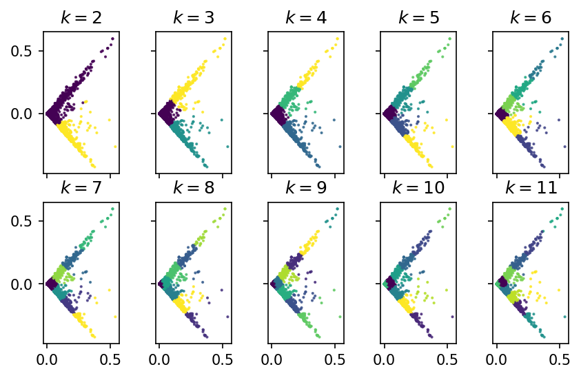
The plots generated above visualizes the dataset clustered into different k clusters. Determining the number of clusters by visualization might not be enough since not enough judgement can be obtained if the following desired characteristics of a good cluster will be considered:
- Compact: points in the same cluster should be close together
- Separated: points not belonging in the cluster should be far from points in the cluster
- Balanced: the number of points in each cluster are comparable
- Parsimonious: the number of cluster should be as few as possible
Compactness of each cluster differs especially as k gets higher. This may be the effect of not removing zero rows in the matrix. There is also no clear separation of clusters. Space between two clusters is zero. In terms of balancing, the datasets in one cluster is not the same with other clusters especially as k gets higher.
Finding Optimal Number of Clusters Using Internal Validation
Internal validation criteria were used to find the optimal number of cluster since we are not relying on ground truth values to evaluate the quality of the clustering. Plots of Sum of squares distances to centroids, Calinski-Harabasz index, Intracluster to intercluster distance ratio, Silhouette coefficient were generated using the function below.
def plot_internal(inertias, chs, iidrs, scs):
    """Plot internal validation values"""
    fig, ax = plt.subplots(1,4, figsize=(18,4))
    ks = np.arange(2, len(inertias)+2)
    ax[0].plot(ks, inertias, '-o', label='SSE');
    ax[0].legend();
    ax[0].set_xlabel('$k$');
    ax[0].set_title('SSE');
    ax[1].plot(ks, chs, '-ro', label='CH');
    ax[1].set_xlabel('$k$');
    ax[1].set_title('CH');
    ax[1].legend();
    ax[2].plot(ks, iidrs, '-go', label='Inter-intra');
    ax[2].set_title('Inter-Intra');
    ax[2].legend();
    ax[2].set_xlabel('$k$');
    ax[3].plot(ks, scs, '-ko', label='Silhouette coefficient');
    ax[3].legend();
    ax[3].set_xlabel('$k$');
    ax[3].set_title('Silhouette Coefficient');
    return ax
plot_internal(res_title['inertias'], res_title['chs'],
              res_title['iidrs'], res_title['scs']);
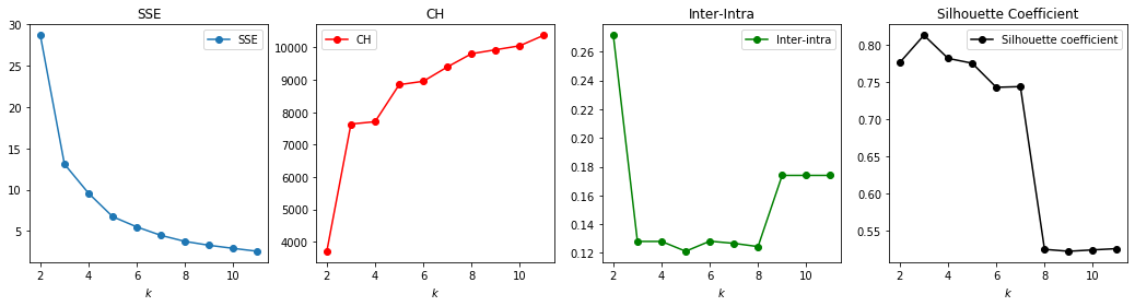
The different plots above provide guidance in choosing the optimal number of k. Based on SSE and CH, the elbow point tells the optimal k. The lowest k giving the lowest Inter/Intra ratio will be the optimal k. For Silhouette coefficient, k that generates high SC is the optimal k.
Based on this criteria, k ranges from 3 to 7. Different iterations were performed to determine if no overlap of dataset occurs among clusters.
# K-means to partition the points into 7 clusters,
# which is the number of clusters based on internal validation criteria
kmeans_title = KMeans(n_clusters=7, random_state=1337,
                      n_init=15, max_iter=1000, tol=1e-6)
y_predict = kmeans_title.fit_predict(bow_title.todense())
Results
The generated clusters are shown below.
df_cluster = pd.DataFrame()
df_cluster['title_lower'] = df_new['title_lower']
df_cluster['group'] = y_predict
group0 = df_cluster[df_cluster['group'] == 0]['title_lower'].tolist()
group1 = df_cluster[df_cluster['group'] == 1]['title_lower'].tolist()
group2 = df_cluster[df_cluster['group'] == 2]['title_lower'].tolist()
group3 = df_cluster[df_cluster['group'] == 3]['title_lower'].tolist()
group4 = df_cluster[df_cluster['group'] == 4]['title_lower'].tolist()
group5 = df_cluster[df_cluster['group'] == 5]['title_lower'].tolist()
group6 = df_cluster[df_cluster['group'] == 6]['title_lower'].tolist()

topic = pd.DataFrame(
    [group0, group1, group2, group3, group4, group5, group6]).T
topic.columns = ['Topic 1', 'Topic 2', 'Topic 3', 'Topic 4',
                 'Topic 5', 'Topic 6', 'Topic 7']
wordcloud1 = WordCloud(max_font_size=50, max_words=200, colormap='Dark2',
                       background_color="white").\
    generate(' '.join(df_cluster[df_cluster['group'] == 0]['title_lower']))
wordcloud2 = WordCloud(max_font_size=50, max_words=200, colormap='Dark2',
                       background_color="white").\
    generate(' '.join(df_cluster[df_cluster['group'] == 1]['title_lower']))
wordcloud3 = WordCloud(max_font_size=50, max_words=200, colormap='Dark2',
                       background_color="white").\
    generate(' '.join(df_cluster[df_cluster['group'] == 2]['title_lower']))
wordcloud4 = WordCloud(max_font_size=50, max_words=200, colormap='Dark2',
                       background_color="white").\
    generate(' '.join(df_cluster[df_cluster['group'] == 3]['title_lower']))
wordcloud5 = WordCloud(max_font_size=50, max_words=200, colormap='Dark2',
                       background_color="white").\
    generate(' '.join(df_cluster[df_cluster['group'] == 4]['title_lower']))
wordcloud6 = WordCloud(max_font_size=50, max_words=200, colormap='Dark2',
                       background_color="white").\
    generate(' '.join(df_cluster[df_cluster['group'] == 5]['title_lower']))
wordcloud7 = WordCloud(max_font_size=50, max_words=200, colormap='Dark2',
                       background_color="white").\
    generate(' '.join(df_cluster[df_cluster['group'] == 6]['title_lower']))

# Display the generated image:
fig, ax = plt.subplots(3, 3, dpi=300);
ax[0][0].imshow(wordcloud1, interpolation='bilinear');
ax[0][0].axis("off");
ax[0][0].set_title("Topic 1: Online Recommendations",fontsize=6);
ax[0][1].imshow(wordcloud2, interpolation='bilinear');
ax[0][1].axis("off");
ax[0][1].set_title("Topic 2: The Democrats",fontsize=6);
ax[0][2].imshow(wordcloud3, interpolation='bilinear');
ax[0][2].axis("off");
ax[0][2].set_title("Topic 3: Today I Learned...",fontsize=6);
ax[1][0].imshow(wordcloud4, interpolation='bilinear');
ax[1][0].axis("off");
ax[1][0].set_title("Topic 4: Customer Support",fontsize=6);
ax[1][1].imshow(wordcloud5, interpolation='bilinear');
ax[1][1].axis("off");
ax[1][1].set_title("Topic 5: Gaming",fontsize=6);
ax[1][2].imshow(wordcloud6, interpolation='bilinear');
ax[1][2].axis("off");
ax[1][2].set_title("Topic 6: New Year",fontsize=6);
ax[2][1].imshow(wordcloud7, interpolation='bilinear');
ax[2][1].axis("off");
ax[2][1].set_title("Topic 7: Donald Trump",fontsize=6);
ax[2][0].axis("off");
ax[2][2].axis("off");
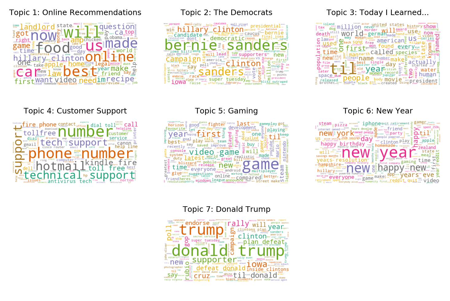
The 7 topics generated gives a significant insight about the dataset. The titles may have been published between December 2016 to January 2017 when Donald Trump had just won the US Elections back in November 2016. There was also an emergence of an online debate whether Sanders could have been a better candidate than Clinton for the Democratic Party. These two clusters indicates that one of the most talked about topic of Reddit users is politics.
Another insight is online users treat Reddit as a platform where they can ask for any advice especially on food and cars, as evident in the number of titles classified under Online Recommendations as shown in the figure below.
Today I Learned cluster suggests also that Reddit users utilize the website in sharing something new. This cluster is the second largest next to the first topic.
Gaming will also be one of the most-taked about topic in the online community especially now that technology is continuously evolving.
Online users also react on different events happening, especially on the most recent one, as shown in Topic 6.
plt.hist(y_predict,histtype='barstacked');
plt.xticks(np.arange(7),('Online Recommendations','The Democrats',
                         'Today I Learned', 'Customer Support','Gaming',
                         'New Year','Donald Trump'),rotation=70);
plt.ylabel('Number of Titles');
plt.title('Distribution of Titles Among Generated Clusters');
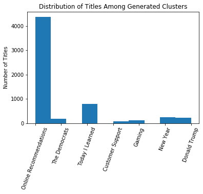
Looking at the histogram shown above, it can be observed that there is still imbalance of datasets per cluster. This means that the obtained results are general topics and can be further improved by using different methods of clustering or further processing of dataset.
Sentiment Analysis Using NLTK
Sentiment analysis using NLTK was used to determine how people are reacting based on the titles. Since the topics were already identified out of clustering, tone of each post is now analyzed using SentimentIntensityAnalyzer, an unsupervised learning algorithm that computationally identifies and categorizes text into three sentiments: positive, negative, or neutral.
Some codes were obtained from Brendan Martin’s GitHub account.
from nltk.sentiment.vader import SentimentIntensityAnalyzer as SIA

sia = SIA()
results = []
for line in df_new['title_lower'].tolist():
    pol_score = sia.polarity_scores(line)
    pol_score['title'] = line
    results.append(pol_score)
df_pol = pd.DataFrame(results)
df_pol.head()
| compound | neg | neu | pos | title | |
|---|---|---|---|---|---|
| 0 | 0.4019 | 0.0 | 0.649 | 0.351 | 7 interesting hidden features of apple ios9 |
| 1 | 0.0000 | 0.0 | 1.000 | 0.000 | need an advice on gaming laptop |
| 2 | 0.0000 | 0.0 | 1.000 | 0.000 | semi automatic ropp capping machine ropp cap ... |
| 3 | 0.0000 | 0.0 | 1.000 | 0.000 | microsoft plumbs oceans depths to test underwa... |
| 4 | 0.0000 | 0.0 | 1.000 | 0.000 | oppo f1 chnh hng fptshopcomvn |
The titles were classified into three based on the compound, a number that scores the sentiment. Titles were tagged positive if compound is above 0.5 while negative for compound less than -0.5. Those in between were tagged neutral.
df_pol['label'] = 0
df_pol.loc[df_pol['compound'] > 0.5, 'label'] = 1
df_pol.loc[df_pol['compound'] < -0.0, 'label'] = -1
df_pol.head()
| compound | neg | neu | pos | title | label | |
|---|---|---|---|---|---|---|
| 0 | 0.4019 | 0.0 | 0.649 | 0.351 | 7 interesting hidden features of apple ios9 | 0 |
| 1 | 0.0000 | 0.0 | 1.000 | 0.000 | need an advice on gaming laptop | 0 |
| 2 | 0.0000 | 0.0 | 1.000 | 0.000 | semi automatic ropp capping machine ropp cap ... | 0 |
| 3 | 0.0000 | 0.0 | 1.000 | 0.000 | microsoft plumbs oceans depths to test underwa... | 0 |
| 4 | 0.0000 | 0.0 | 1.000 | 0.000 | oppo f1 chnh hng fptshopcomvn | 0 |
The following are the results generated after classifying the titles into three sentiments.
print("Positive titles:\n")
for i in list(df_pol[df_pol['label'] == 1].title)[:5]:
    print(i)

print("\nNegative titles:\n")
for j in list(df_pol[df_pol['label'] == -1].title)[:5]:
    print(j)
Positive titles:

sfnyc what is the best way to find a good startup lawyer
id like to buy the rights of a post on reddit to recreate in another medium how do i create a legal contract for this between strangers online
aussie heroes steam group
happy 2016 and may all your games be mostly bug free
i have a great idea for a trpg

Negative titles:

california is it a crime when a religious figure lecturer has relations with one of his followers
being accused of public indecency among other things this is a misunderstanding because i had health issues kansas usa
charged with dui 2 years and 4 months after i was involved in a single car accident
new poll shows how far hillary has fallen with democrats
how cod kills your hope
Word Polarity Distribution
To determine the distribution of the sentiments, a distribution plot was generated below.
print(df_pol.label.value_counts(normalize=True) * 100)
fig, ax = plt.subplots(figsize=(5, 3))
counts = df_pol.label.value_counts(normalize=True) * 100
sns.barplot(x=counts.index, y=counts, ax=ax)

ax.set_xticklabels(['Negative', 'Neutral', 'Positive'])
ax.set_ylabel("Percentage")
ax.set_title('Classification of Sentiments')
plt.show()
 0    64.527421
-1    23.537256
 1    11.935323
Name: label, dtype: float64
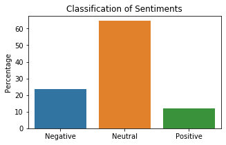
It can be observed that 64.52% of the titles are neutral in nature. But interestingly, there are a lot of negative titles compared to positive ones. The distribution may have been affected by the events that happened during the time these titles were published.
Classification of Words
To dig deeper into the sentiments of the users, the words per sentiment type were obtained.
pos_lines = list(df_pol[df_pol.label == 1].title)
neg_lines = list(df_pol[df_pol.label == -1].title)
neut_lines = list(df_pol[df_pol.label == 0].title)

wc1 = WordCloud(max_font_size=50, max_words=50, colormap='Dark2',
                       background_color="white").\
    generate(' '.join(pos_lines))
wc2 = WordCloud(max_font_size=50, max_words=50, colormap='Dark2',
                       background_color="white").\
    generate(' '.join(neg_lines))
wc3 = WordCloud(max_font_size=50, max_words=50, colormap='Dark2',
                       background_color="white").\
    generate(' '.join(neut_lines))

fig, ax = plt.subplots(1, 3, dpi=300);
ax[0].imshow(wc1, interpolation='bilinear');
ax[0].axis("off");
ax[0].set_title("Positive",fontsize=6);
ax[1].imshow(wc2, interpolation='bilinear');
ax[1].axis("off");
ax[1].set_title("Negative",fontsize=6);
ax[2].imshow(wc3, interpolation='bilinear');
ax[2].axis("off");
ax[2].set_title("Neutral",fontsize=6);
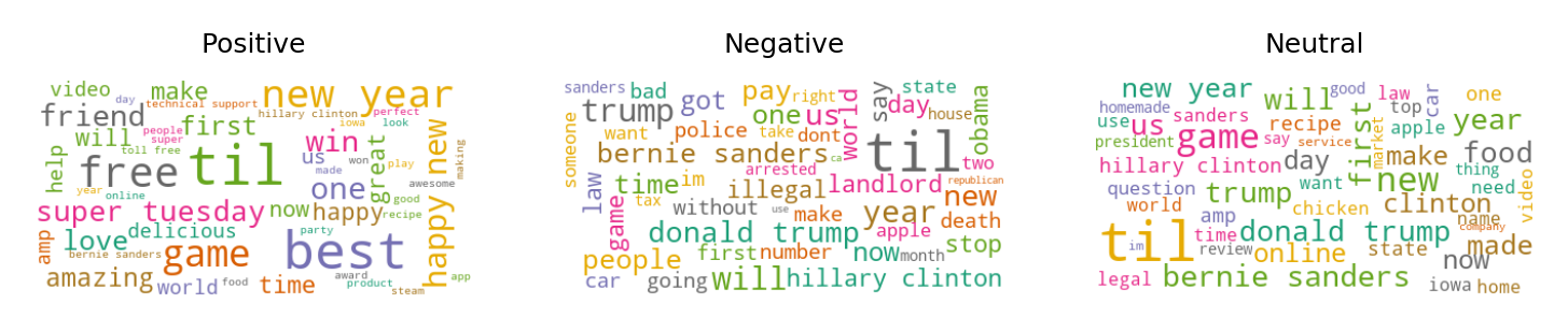
It can be observed that positive titles talk about new year and gaming. Negative titles are associated with US politics, giving an insight that Reddit users have negative sentiment on the outcome of the US elections. One of the negative words shown in the word cloud is ‘Trump’, who happened to be the newly elected US president during the time the titles were published online.
Another interesting observation is the word TIL appears on all clusters. This means that there are underlying subgroups within those titles containing the word TIL. Additional clustering can be done on these titles.
Conclusion
The performed K-means clustering algorithm was able to generate possible subreddits out of the given datasets. However, generated topics are somehow general in nature and datasets are imbalanced. Thus, it can be concluded that K-means clustering can be used to group a dataset by general topics. The sentiment analysis using NLTK was able to determine the mood of the authors in writing the title.
Over-all, the two methods performed did not only generate clusters but generated meaningful insights on what was happening during the time when the Reddit titles were generated and most significantly, reactions of Reddit users were identified. From the dataset analyzed, it was concluded that users have negative views the US Presidential Elections 2016.
Recommendations
Based on the results obtained, the following recommendations are suggested to further improve the study.
- Perform other word processing techniques such as lemmatization or stemming to further enhance clustering and remove overlap of dataset as seen in the results above.
- Consider to include non-ASCII characters in clustering or translate non-English words to English.
- Use of other clustering methods is recommended to further validate the number of clusters obtained.
- Consider to cluster the titles clustered under the TIL group to further breakdown topics into more specific subgroups.
Acknowledgment
The success and final outcome of this project required a lot of guidance and assistance from the MS Data Science faculty particularly Prof. Erika Legara, Prof. Christian Alis and Engr. Eduardo David Jr. who granted permission to use all required equipment and the necessary materials to complete the tasks.
Deep gratitude is also given to AIM’s Analytics, Computing, and Complex Systems Laboratory for providing the opportunity to do the project work using the laboratory’s supercomputer.
Special thanks is given to MSDS 2020 students (to be revealed after checking of this project) who collaborated with the user in conceptualizing the framework of the report.
References
[1] A beginner’s guide to Reddit (link)
[2] Alis, C. Representative-based clustering.ipynb
[3] Martin, B. Sentiment Analysis on Reddit News Headlines with Python’s Natural Language Toolkit (NLTK). (link)
[4] Tripathi, M. How to process textual data using TF-IDF in Python (link)
[5] Brownlee, J. How to Prepare Text Data for Machine Learning with scikit-learn (link)
[6] Ganesan, K. How to Use Tfidftransformer & Tfidfvectorizer? (link)
[7] StackOverflow